Photoacoustic image reconstruction using backward projection

In photoacoustic tomography (PAT), laser pulses are delivered into biological tissue, which are to be absorbed, particularly by the blood vessels. Ultrasonic waves are consequently produced via thermo-elastic expansion. By projecting the ultrasonic wave backward toward the tissue, the initial ultrasonic pressure distribution can be recognized, rendering a photoacoustic image. The process of backward projection is similar to time-reversal. However, as opposed to marching in the time-domain, the backward projection marches in the direction normal to the receiver plane. Additionally, there is no need to reverse the signal in time in the process of backward projection. The forward propagation of the emitted ultrasonic wave from the source is simulated with the k-Wave toolbox. The received signals are backward projected with the mSOUND toolbox for the image reconstruction.

Forward propagation with k-Wave

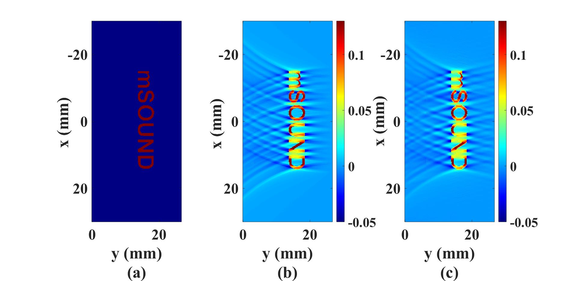
The forward propagation of the emitted ultrasonic wave from the source is simulated with the k-Wave toolbox. An initial source with the ‘mSOUND’ shape is used in this example.


% define the computational domain   
Nx = 800;   % number of grid points in the x-direction
Ny = 300;   % number of grid points in the y-direction
dx = 1.3393e-04;   % [m]   
dy = 1.3393e-04;   % [m]   
kgrid = makeGrid(Nx, dx, Ny, dy);
dt = 1.1161e-08;   % [s]   
kgrid.t_array = 0:dt:3.4286e-05; 

% assign the properties of the propagation medium   
medium.sound_speed = 1500*ones(Nx, Ny);
medium.BonA        = 2.0*(0-1.0);
medium.density     = 1000*ones(Nx, Ny);
medium.alpha_coeff = 0.0; 
medium.alpha_power = 2.0;

% define source and sensor   
load mSOUND_logo.mat   % load the initial source distribution   
p0 = 1; 
source.p = p0;
source.p_mask = s;
sensor.mask = zeros(Nx, Ny); 
sensor.mask(:, 250) = 1; 

% excitation signal   
sample_freq = 1/dt;  [Hz] 
signal_freq = 1e6;   [Hz] 
source_mag = p0;     [Pa] 

% set the input options  
input_args = {'DisplayMask', sensor.mask, 'DataCast', 'single',...
                 'PlotScale',[-source_mag/2, source_mag/2]};
sensor.record = {'p'};

% run the simulation with k-Wave  
sensor_data = kspaceFirstOrder2D(kgrid, medium, source, sensor, input_args{:});
kwave_P_time = reshape(sensor_data.p, Nx, length(kgrid.t_array));

Backward simulation

The source_p required for the function Backward2D is the signals recorded on the linear array located at the right boundary of Figure (a) above, generated by k-Wave.


clear medium
medium.c0 = 1500; % reference speed of sound [m/s]    

% define the computational domain   
num_x = Nx;    % number of grid points in the x-direction
num_y = 200;   % number of grid points in the y-direction
dt = 8*dt;     % time step in TMDM [s] 
x_length = num_x*dx; 
y_length = num_y*dy;
t_length = kgrid.t_array(end); 

mgrid = set_grid(dt, t_length, dx, x_length, dy, y_length);

% define the computational domain   
source_p = kwave_P_time(:, 1:8:end).';

% assign the properties of the propagation medium   
medium.c    = 1500;
medium.rho  = 1000;
medium.beta = 0;
medium.ca   = 0;
medium.cb   = 2.0;
medium.NRL_gamma = 0.9;
medium.NRL_alpha = 0.009;

% backward projection with TMDM to reconstruct the initial source distribution  
sensor_mask = ones(mgrid.num_x, mgrid.num_y+1);
p = Backward2D(mgrid, medium, source_p, sensor_mask, 0, 'NRL');

Figure (b) below shows the reconstructed image with the time-reversal algorithm in k-Wave and Fig. (c) below shows the reconstructed image using the backward projection in mSOUND. There is a fine agreement between these two results. source image reconstruction

Other examples