Simulation of a 3D homogeneous medium using the transient mixed domain method
This example shows how to simulate the wave propagation in a 3D homogeneous medium with the transient mixed domain method. A focused beam is studied in this example.
Generating the grid structure to define the computational domain
To define the temporal and spatial computational domains in 3D forward simulations, the funciton set_grid is used.For 3D problems, eight inputs are required to call this function. Coordinates generated with this function are all in Cartesian coordinates. We assume the z-axis is perpendicular to the transducer surface. The spatial resolution should in principle be a small fraction of the wavelength (e.g., 1/4 of the wavelength). The temporal resolution should at least satisfy the Nyquist criteria.
dx = 3.75e-04;    % step size in the x direction [m]
dy = 3.75e-04;    % step size in the y direction [m]
dz = 3.75e-04;    % step size in the z direction [m]
dt = 6.25e-08;    % time step size [s]

x_length = 0.0300;     % computational domain size in the x direction [m]
y_length = 0.0300;     % computational domain size in the y direction [m]
z_length = 0.0210;     % computational domain size in the z direction [m]
t_length = 1.60e-05;   % temporal domain size [s]
mgrid = set_grid(dt, t_length, dx, x_length, dy, y_length, dz, z_length);
Defining a 3D phased array transducer
In this example, a phased array transducer is used to generate the focused ultrasound beam.
p0 = 1.0e6;    % source pressure magnitude [Pa]
TR_focus  = 0.0120;    % transducer focal length [m]
TR_radius = 0.0075;    % transducer aperture radius [m]

% calculate the phase delay
X = (ones(mgrid.num_y,1)*mgrid.x).';
Y = ones(mgrid.num_x,1)*mgrid.y;
delay = sqrt(X.^2 + Y.^2 + TR_focus^2)/medium.c0;
delay = delay - min(min(delay));
Excitation signal
A four-cycle Gaussian-modulated pulse is used as the excitation signal.
% define the pulse length [s]
ts = [-4/fc:dt:4/fc].';
% allocate space for excitation signal
source_p = zeros(length(ts), mgrid.num_x, mgrid.num_y);

% assign signal to each source element
for cel1 = 1:mgrid.num_x
    for cel2 = 1:mgrid.num_y
        source_p(:, cel1, cel2) = ...
           sin(2*pi*fc*(ts+delay(cel1, cel2))).*...
           exp(-(ts+delay(cel1, cel2)).^2*fc^2/2);
    end
end

% generate a circular transducer
RHO = sqrt(X.^2+Y.^2);
source_p(:, RHO>TR_radius) = 0;
Defining the medium properties
A nonlinear homogeneous medium with attenuation is defined. For 3D simulations, the medium properties should be given as matrices with a size (mgrid.num_x, mgrid.num_y, mgrid.num_z+1). For homogeneous media, though, the medium properties can be described by a single scalar. medium.c0 is the reference speed of sound and generally, it is chosen as the minimum value of medium.c.
medium.c    = 1500;    % speed of sound [m/s]
medium.rho  = 1000;    % density [kg/m^3]
medium.beta = 3.6;     % nonlinearity coefficient
medium.ca   = 0.005;   % attenuation coefficient [dB/(MHz^y cm)]
medium.cb   = 2.0;     % power law exponent
3D forward simulation
The acoustic pressure field is calculated with the 3D forward simulation function Forward3D.
% define where the pressure will be recorded
sensor_mask = zeros(mgrid.num_x, mgrid.num_y, mgrid.num_z+1);
sensor_mask(40:120, 40:120, 2:end) = 1;

% 3D forward simulation
p_total = Forward3D(mgrid, medium, excit_ps, sensor_mask, 0);
The time-domain and freuqency-domain signals recorded at the transducer focus are shown in the figures below.
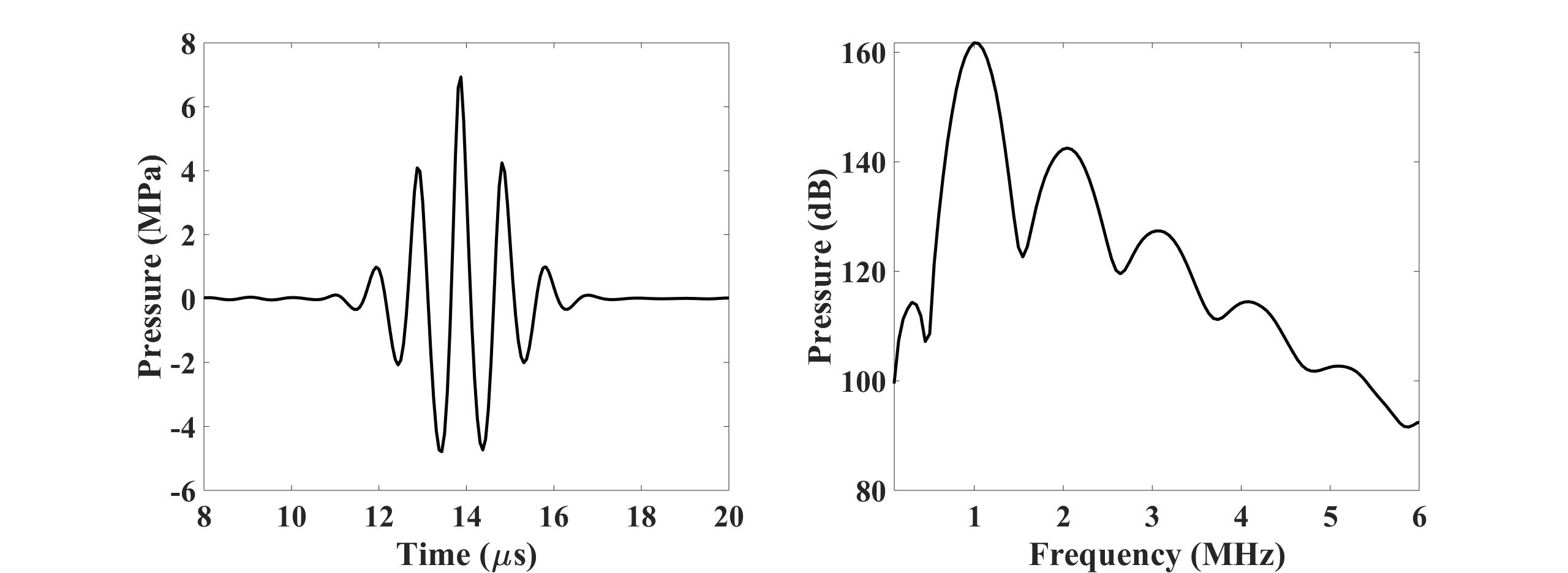 The acoustic signal recorded at the transducer focus as well as its Fourier components are shown in the two figures above.
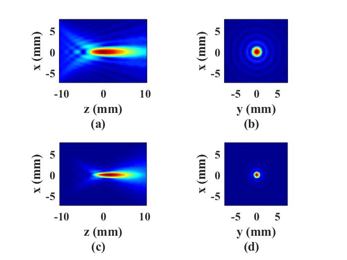
The pressure fields at the fundamental (top) and the second harmonic frequencies (bottom) are shown below. The two figures on the left
show the pressure fields on the xz plane while the two figures on the right show the pressure fields on the xy plane.
The acoustic signal recorded at the transducer focus as well as its Fourier components are shown in the two figures above.
The pressure fields at the fundamental (top) and the second harmonic frequencies (bottom) are shown below. The two figures on the left
show the pressure fields on the xz plane while the two figures on the right show the pressure fields on the xy plane.
Other examples
·
Simulation of a 2D homogeneous medium using the transient mixed domain method
·
Simulation of a 2D heterogeneous medium using the transient mixed domain method
·
Simulation of a strongly 2D heterogeneous medium using the transient mixed domain method
·
Simulation of a 3D homogeneous medium using the transient mixed domain method
·
Selecting the proper temporal domain size for the TMDM
·
Shock wave simulations with TMDM
·
Simulation of a 2D homogeneous medium using the frequency-specific mixed domain method
·
Simulation of a 2D heterogeneous medium using the frequency-specific mixed domain method
·
Simulation of a 3D homogeneous medium using the frequency-specific mixed domain method
·
Simulation of a 3D heterogeneous medium using the frequency-specific mixed domain method
·
Reducing the spatial aliasing error using the non-reflecting layer
·
Comparing pressure release and rigid boundary conditions
·
Image reconstruction using backward projection
·
Reconstruction of the source pressure distribution with FSMDM in a 3D homogeneous medium
·
Integrating mSOUND with k-Wave for transducers of arbitrary shape
·
Integrating mSOUND with FOCUS for transducers of arbitrary shape
·
Integrating mSOUND with k-Wave for thermal simulations