Simulation of a strongly 2D heterogeneous medium using the transient mixed domain method

This example demonstrates how to use the transient mixed domain method (TMDM) for simulating wave propagation in 2D, strongly heterogeneous media. For strongly heterogeneous media (e.g., skulls), phase and amplitude corrections are needed as the original mixed domain method only applies to weakly heterogeneous media (in terms of speed of sound and density variations). This example shows how to apply these corrections. Generally, for simulations of heterogeneous media with small speed of sound or density contrast (contrast ratio being less than 1.05), it is unnecessary to apply corrections.

Generating the grid structure to define the computational domain

We first need to define the temporal and spatial computational domains in 2D forward simulations with the funciton set_grid. For 2D problems, six inputs are required to call this function. Coordinates defined within the mgrid structure are all in the Cartesian coordinates. The spatial resolution should in principle be a small fraction of the wavelength (e.g., 1/4 of the wavelength). The temporal resolution should at least satisfy the Nyquist criteria.

        
dx = 5.3571e-04;   % step size in the x direction [m] 
dy = 1.3393e-04;   % step size in the y direction [m] 
dt = 1.1905e-07;   % time step size [s] 

x_length = 0.1671;      % computational domain size in x direction [m] 
y_length = 0.0857;      % computational domain size in y direction [m] 
t_length = 6.8571e-05;  % temporal domain size [s] 
mgrid = set_grid(dt, t_length, dx, x_length, dy, y_length);

Defining the medium properties

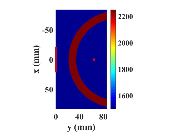
The transducer setting in this case is similar to the example Simulation of a 2D homogeneous medium using the transient mixed domain method. In this example, the speed of sound contrast and density contrast are all 1.5. The 2D model used in this example is shown in the figure below.

 
p0 = 1.0e6;   % source pressure magnitude [Pa]  
fc = 0.7e6;   % fundamental frequency [Hz]  
TR_focus  = 0.0643;   % transducer focal length [m]         
TR_radius = 0.0214;   % Transducer radius [m] 

load 2D_strongly_heterogeneous_model.mat  % load the tissue model data   
medium.c    = c;      % speed of sound [m/s]      
medium.rho  = rho;    % density [kg/m^3]             
medium.beta = beta;   % nonlinearity coefficient     
medium.ca   = ca;     % attenuation coefficient [dB/(MHz^y cm)]     
medium.cb   = cb;     % power law exponent

2D forward simulation

The acoustic pressure field is calculated with the function Forward2D. Corrections are applied in this example because of the strong speed of sound and density contrast. Reflections up to the fourth-order are also included in this simulation.


% define where the pressure will be recorded  
sensor_mask = zeros(mgrid.num_x, mgrid.num_y+1);
sensor_mask(100:300, 2:end) = 1;

% the maximum order of reflection included in the simulation  
reflection_order = 4; 

% 2D forward simulation  
p_total = Forward2D(mgrid, medium, source_p, sensor_mask,...
          reflection_correction, 'correction');

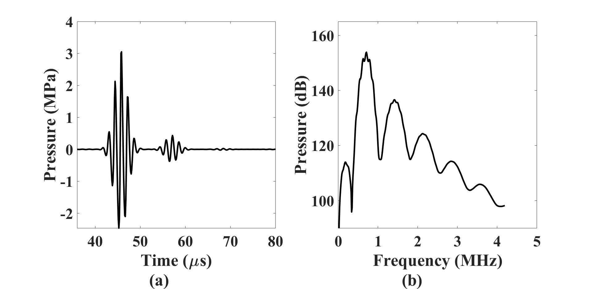
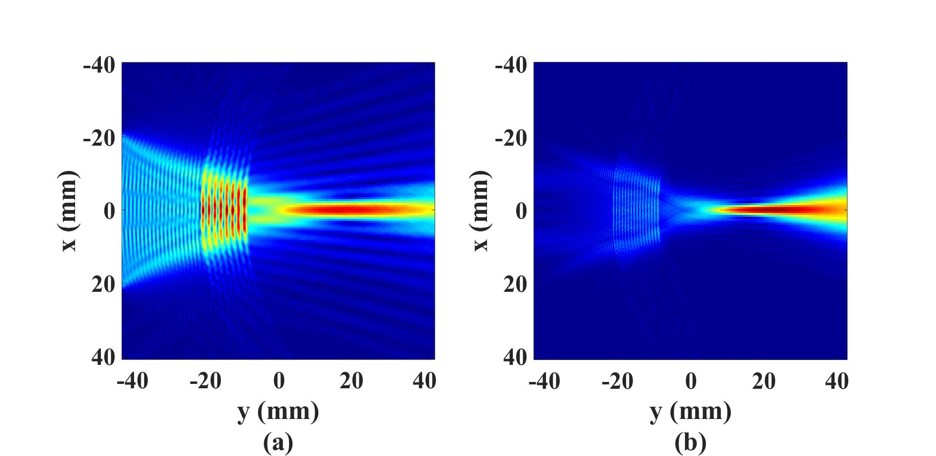
The figure below shows the (a) waveform and (b) frequency-domain spectrum for the signal recorded at the transducer focal point. (a) time-domain and (b) frequency-domain signal at the transducer focus The figure below shows the acoustic pressure field (a) at the fundamental and (b) at the second-harmonic frequency.

Other examples