Integrating mSOUND with k-Wave for thermal simulations

This example shows how to combine mSOUND and k-Wave for thermal simulations. The acoustic simulation is conducted with mSOUND first and the thermal simulation is subsequently implemented by k-Wave.

Acoustic simulation

The acoustic simulation is first conducted with function Forward2D_fund, to generate the pressure field P_fundamental for the subsequent thermal simulation. In the thermal simulation, the pressure on the source plane will be excluded. Then we need to extract the pressure amplitdue from the acoustic simulation result P_fundamental. The output pressure P_fundamental includes the values at the source plane. In the thermal simulation, the pressure at the source plane will be excluded, otherwise there is a mismatch in the size of the matrices used in mSOUND and k-Wave.

 
% define the computational domain 
x_length = 0.0451;  % computational domain size in the x direction [m] 
y_length = 0.0450;  % computational domain size in the y direction [m] 
dx = 1.5000e-04;  % step size in the x direction [m] 
dy = 1.5000e-04;  % step size in the y direction [m]
mgrid = set_grid(0, 0, dx, x_length, dy, y_length);

TR_focus = 0.0360;  % transducer focal length    
TR_radius = 0.0090; % transducer aperture radius 

% calculate the phase delay     
delay = sqrt((mgrid.x).^2 + (TR_focus)^2)/medium.c0;  % [s]
delay = delay - min(delay);

p0 = 0.8e6; % pressure magnitude at the source [Pa]  
fc = 1.0e6;	% fundamental frequency	[Hz]    
omega_c = 2*pi*fc; % angular frquency [rad/s]   
source_p = p0*exp(1i*omegac*delay);  % define the pulse   
source_p(abs(mgrid.x)>TR_radius) = 0;

medium.c0   = 1500; % reference speed of sound [m/s] 
medium.c    = 1500; % speed of sound [m/s]      
medium.rho  = 1000; % density [kg/m^3]             
medium.beta = 0;    % nonlinearity coefficient     
medium.ca   = 0.75; % attenuation coefficient [dB/(MHz^y cm)]        
medium.cb   = 1.5;  % power law exponent 

% non-reflecting layer 
medium.absorb_gamma = 0.5;
medium.absorb_alpha = 0.05;

% forward wave propagation     
P_fundamental = Forward2D_fund(mgrid, medium, source_p, omega_c, 0, 'NRL');
% extract the pressure amplitude and exclude the values on the source plane    
p = abs(P_fundamental(:,2:end));

Thermal simulation

Thermal simulation is conducted with k-Wave.

  
% convert the absorption coefficient to nepers/m 
alpha_np = db2neper(medium.ca, medium.cb) * (omegac).^medium.cb;
% calculate the volume rate of heat deposition 
Q = alpha_np .* p.^2 ./ (medium.rho .* medium.c);
% set the background temperature and heating term 
source.Q = Q;
source.T0 = 37;

% define medium properties related to diffusion 
medium.density = 1000;  % [kg/m^3] 
medium.thermal_conductivity = 0.5; % [W/(m.K)] 
medium.specific_heat = 3600; % [J/(kg.K)]  
% create the computational grid  
kgrid = kWaveGrid(mgrid.num_x, mgrid.dx, mgrid.num_y, mgrid.dy); 
% create kWaveDiffusion object  
kdiff = kWaveDiffusion(kgrid, medium, source, []);
 
on_time  = 10; % source on time [s]  
off_time = 20; % source off time [s]  
dt = 0.1; % set time step size [s]  

% take time steps    
kdiff.takeTimeStep(round(on_time / dt), dt);   
T1 = kdiff.T; % store the current temperature field    

% turn off heat source and take time steps    
kdiff.Q = 0; 
kdiff.takeTimeStep(round(off_time / dt), dt);
% store the current temperature field  
T2 = kdiff.T;

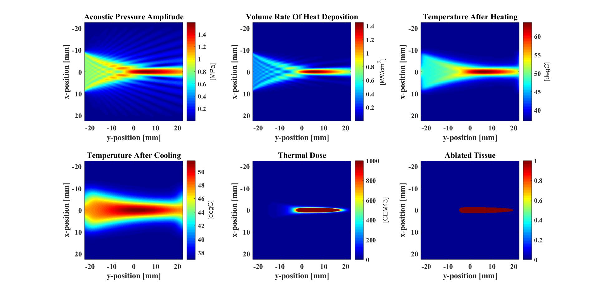
The figures below show the acoustic and thermal simulation results. The acoustic simulation is conducted with mSOUND and the thermal simulation is conducted with k-Wave. The resulting pressure, volume rate of heat deposition,
temperature field, thermal dose, and ablation volume

The resulting pressure, volume rate of heat deposition,
temperature field, thermal dose, and ablation volume

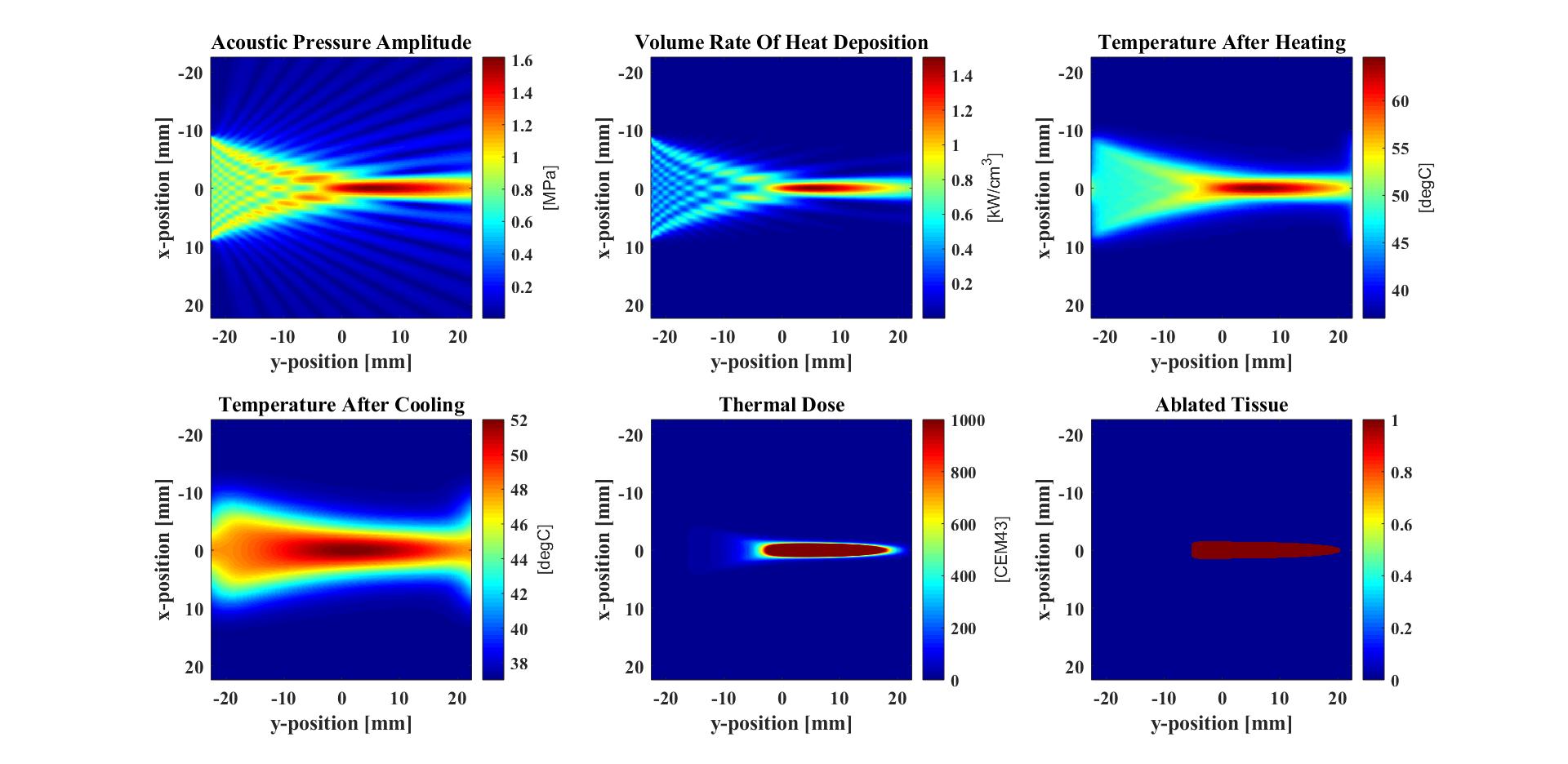
The figures below show the acoustic and thermal simulation results. Both the acoustic and thermal simulations are conducted with k-Wave. The resulting pressure, volume rate of heat deposition,
temperature field, thermal dose, and ablation volume

Other examples