Simulation of a 3D homogeneous medium using the frequency-specific mixed domain method
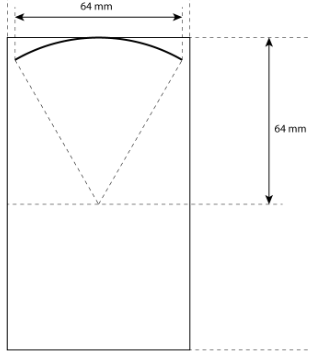
This example shows how to simulate the wave propagation in a 3D homogeneous and lossy medium with the frequency-specific mixed domain method. In this example, we model a bowl transducer by approximating it as a 2D phased array. The bowl transducer has a diameter and radius of curvature both being 64 mm, as shown in the figure below.
Generating the grid structure to define the computational domain
We first need to define the temporal and spatial computational domains in 3D forward simulations.
In FSMDM, any arbitrary values can be set for the time step and temporal domain size, since they are not being used.
Here, we set them to 0. We also define the background acoustic medium in this section.
medium.c0 = 1500;       % speed of Sound [m/s]
medium.rho0 = 1000;     % density of medium [kg/m^3]
medium.beta0 = 3.6;     % nonlinearity coefficient
medium.ca0 = 4;         % attenuation coefficient [dB/(MHz^y cm)]; 1 dB/cm at 500 kHz
medium.cb0 = 2.0;       % power law exponent

dx = lambda/6;   % step size in the x direction [m]
dy = lambda/6;   % step size in the y direction [m]
dz = lambda/6;   % step size in the z direction [m]

x_length = 70e-3*2+dx;   % computational domain size in the x direction [m]
y_length = 70e-3*2+dx;   % computational domain size in the y direction [m]
z_length = 120e-3;       % computational domain size in the z direction [m]

mgrid = set_grid(0, 0, dx, x_length, dy, y_length, dz, z_length);
Excitation signal
Since the simulation is conducted in the frequency domain, a continuous sine wave is assumed as the excitation signal.
Note that in this case, the pressure would be a complex number rather than a real number as in the TMDM.
 % apply phase delay to generate the focused beam
source_p = p0*exp(1i*omega_c*delay);
RHO = sqrt(X.^2+Y.^2);
% apply spatial truncation to construct a circular transducer
source_p(RHO>TR_radius) = 0;
Defining the medium properties
Define the homogeneous medium. It is the same as the background medium.
medium.c    = medium.c0;     % speed of sound [m/s]
medium.rho  = medium.rho0;   % density [kg/m^3]
medium.beta = medium.beta0;  % nonlinearity coefficient
medium.ca   = medium.ca0;    % attenuation coefficient [dB/(MHz^y cm)]
medium.cb   = medium.cb0;    % power law exponent
3D forward simulation
The fundamental pressure field is calculated with the 3D forward simulation function Forward3D_fund. The pressure field at the second-harmonic frequency under the quasi-linear approximation (weakly nonlinear wave propagation) is calculated with the function Forward3D_sec.
fc = 0.5e6;        % ultrasound frequency/ Hz
omega_c = 2*pi*fc; % angular frequency
% forward propagation of the wave at the fundamental frequency
P_fundamental = Forward3D_fund(mgrid, medium, source_p, omega_c);

% forward propagation of the wave at the 2nd harmonics
P_second = Forward3D_sec(mgrid, medium, p_fundamental, omega_c);
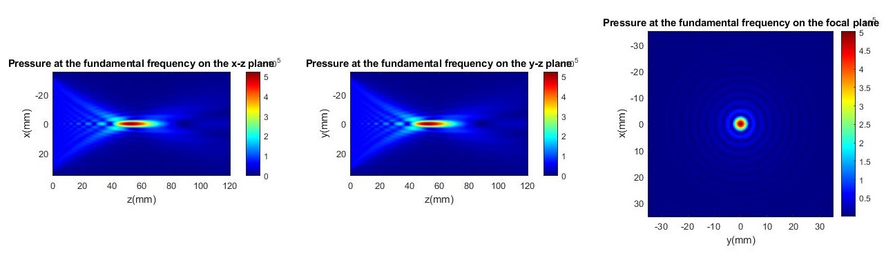
The three figures below show the fundamental frequency pressure field distribution in the
(left) xz plane, (middle) yz plane and (right) xy plane crossing the
focal point.
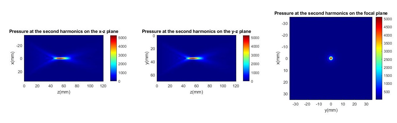
The three figures below show the second-harmonic frequency pressure field distribution in the (left) xz plane, (middle) yz plane and (right) xy plane crossing the focal point. As expected, a smaller focal region can be seen at the 2nd harmonics.
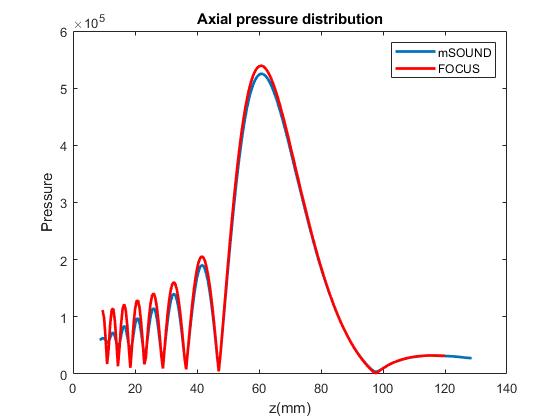
 The figure below shows the comparison between mSOUND and FOCUS for the fundamental frequency pressure distribution along the axial direction.
The difference between the two models is mainly due to the different boundary conditions used. Please see
Comparing rigid boundary condition and pressure release boundary condition for modeling ultrasound transducers for more details. Please also see
Integrating mSOUND with FOCUS for transducers of curved shape on how to exactly model a bowl transducer without making the 2D phased array approximation.
The figure below shows the comparison between mSOUND and FOCUS for the fundamental frequency pressure distribution along the axial direction.
The difference between the two models is mainly due to the different boundary conditions used. Please see
Comparing rigid boundary condition and pressure release boundary condition for modeling ultrasound transducers for more details. Please also see
Integrating mSOUND with FOCUS for transducers of curved shape on how to exactly model a bowl transducer without making the 2D phased array approximation.
Other examples
·
Simulation of a 2D homogeneous medium using the transient mixed domain method
·
Simulation of a 2D heterogeneous medium using the transient mixed domain method
·
Simulation of a strongly 2D heterogeneous medium using the transient mixed domain method
·
Simulation of a 3D homogeneous medium using the transient mixed domain method
·
Selecting the proper temporal domain size for the TMDM
·
Shock wave simulations with TMDM
·
Simulation of a 2D homogeneous medium using the frequency-specific mixed domain method
·
Simulation of a 2D heterogeneous medium using the frequency-specific mixed domain method
·
Simulation of a 3D homogeneous medium using the frequency-specific mixed domain method
·
Simulation of a 3D heterogeneous medium using the frequency-specific mixed domain method
·
Reducing the spatial aliasing error using the non-reflecting layer
·
Comparing pressure release and rigid boundary conditions
·
Image reconstruction using backward projection
·
Reconstruction of the source pressure distribution with FSMDM in a 3D homogeneous medium
·
Integrating mSOUND with k-Wave for transducers of arbitrary shape
·
Integrating mSOUND with FOCUS for transducers of arbitrary shape
·
Integrating mSOUND with k-Wave for thermal simulations