Integrating mSOUND with FOCUS for transducers of curved shape

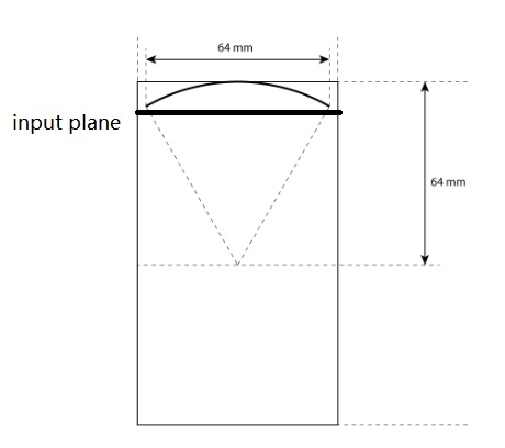
This example shows how to integrate mSOUND with FOCUS for simulations involving curved transducers. Currently, only planar phased-arrays can be directly set up in mSOUND for modeling focused beams. To more accurately model a physically curved transducer, the user can use FOCUS to generate the input plane pressure field (right in front of the edge of the transducer), which would then be used in mSOUND to further propagate the wave. In this example, a 3D bowl transducer is first modeled with FOCUS and then with mSOUND. The diameter of the bowl transducer is 64 mm. The radius of curvature is also 64 mm. It is the same transducer as used in Simulation of a 3D homogeneous medium using the frequency-specific mixed domain method.

Generating the grid structure to define the computational domain

We first need to define the temporal and spatial computational domains in 3D forward simulations. In FSMDM, any arbitrary values can be set for the time step and temporal domain size, since they are not being used. Here, we set them to 0. We also define the background acoustic medium in this section.

      

medium.c0 = 1500;       % speed of Sound [m/s] 
medium.rho0 = 1000;     % density of medium [kg/m^3] 
medium.beta0 = 0;     % nonlinearity coefficient      
medium.ca0 = 4;         % attenuation coefficient [dB/(MHz^y cm)]; 1 dB/cm at 500 kHz  
medium.cb0 = 2.0;       % power law exponent   

dx = lambda/6;   % step size in the x direction [m] 
dy = lambda/6;   % step size in the y direction [m] 
dz = lambda/6;   % step size in the z direction [m] 

x_length = 70e-3*4+dx;     % computational domain size in the x direction [m] 
y_length = 70e-3*4+dx;     % computational domain size in the y direction [m] 
z_length = 120e-3-19*dz;   % computational domain size in the z direction [m] 
    
mgrid = set_grid(0, 0, dx, x_length, dy, y_length, dz, z_length);

Excitation signal

The input plane pressure is first generated by FOCUS. The input plane is at the 20th grid point in the z-direction, which is 9.5 mm away from the first grid point (the bottom of the bowl transducer). The corresponding FOCUS code (input_plane_FOCUS_bowl_transducer_code.m) can be found in the example folder. The figure below shows the bowl transducer and the input plane (thick black line).

  
load FOCUS_input_plane_focused_lossy.mat

Defining the medium properties

Define the homogeneous medium. It is the same as the background medium.

 
medium.c    = medium.c0;     % speed of sound [m/s]   
medium.rho  = medium.rho0;   % density [kg/m^3]             
medium.beta = medium.beta0;  % nonlinearity coefficient     
medium.ca   = medium.ca0;    % attenuation coefficient [dB/(MHz^y cm)]     
medium.cb   = medium.cb0;    % power law exponent

3D forward simulation

The pressure field is calculated with the 3D forward simulation function Forward3D_fund.

 
fc = 0.5e6;        % ultrasound frequency/ Hz   
omega_c = 2*pi*fc; % angular frequency   
% forward propagation of the wave at the fundamental frequency    
P_fundamental = Forward3D_fund(mgrid, medium, source_p, omega_c);

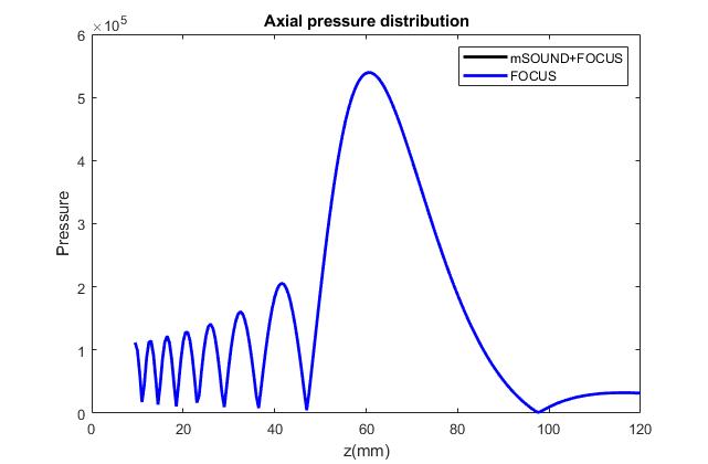
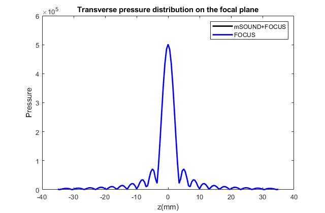
The two figures below show the pressure field distribution along the axial direction and transverse direction (on the focal plane). The results obtained from FOCUS alone are also shown for comparison. Excellent agreement can be observed. Axial pressure field of the bowl transducer

Axial pressure field of the bowl transducer

Transverse pressure field of the bowl transducer

Other examples