Selecting the proper temporal domain size for the TMDM
Normally, it is suggested that the temporal domain size (length of the time axis) should be at least sufficiently large so that the majority of the wave would exit the computational spatial domain. However, this is not a mandatory requirement if the interest is merely to predict the waveform at a certain point in space. Since discrete Fourier transform assumes period functions, when the wave approaches and eventually enters the end of the time axis, it is going to come out from the other side of the axis. Though ultimately this can be considered as an error caused by the under-sampling of the frequency domain, we can leverage this to achieve faster computation. Specifically, the temporal domain size in the TMDM can be chosen to be slightly larger than the pulse length to significantly save the computation time and required memory size. It is noted that, using a small temporal domain size would preclude multiple reflection events that trail behind the main wavefront and lose the track on the arrival time (though the arrival time can be manually calculated for simple scenarios like wave propagation in homogeneous media). Additionally, artificial waveforms will appear in the animation (a similar type of artifact also exists in the spatial domain and can be minimized by absorption layers. Please refer to Reducing the spatial aliasing error using the non-reflecting layer). Therefore, the proper temporal domain size should be carefully chosen based on the specific application that the user has in mind.
Forward propagation
This example is based on the example
Simulation of a 2D heterogeneous medium
using the transient mixed domain method. Two different temporal domain sizes are used and they are
t_length = 8.0e-06 second
and t_length = 3.2e-05 second.
sensor_mask = zeros(mgrid.num_x, mgrid.num_y+1);
sensor_mask(round(mgrid.num_x/2), 113) = 1;
reflection_order = 2;
p_total = Forward2D(mgrid, medium, source_p, sensor_mask,
          reflection_order, 'animation');
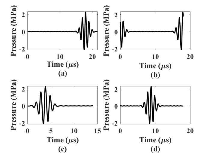
Figures (a)-(c) below show the waveforms at the same position with different temporal domain sizes.
Fig. (a) is with the largest temporal domain size while Fig. (c) is with the smallest temporal domain size.
Fig. (b) clearly shows that the wave enters the very end of the temporal domain and comes out from
the other side. To rearrange Fig. (b) in order to have a physically correct waveform, “fftshift” is applied to the waveform and
Fig. (d) is generated. Note that here, "fftshift" is simply a manipulation that we use to post-process the waveform shown in Fig. (b). There is no physical meaning
of "fftshift" in this context as we are not dealing with FFT here.
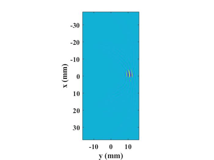
 The first figure below shows the snapshot of the animation for the simulation with t_length = 8.0e-06 second.
The second figure below shows the snapshot of the animation for the simulation with t_length = 3.2e-05 second.
Comparing these two figures, it can be seen that the two wavefronts on the left and in the middle of the first figure are artifacts.
These are in fact two wavefronts occurring at earlier time instants, but are now shown concurrently with the true wavefront.
In terms of the computation time, the first simulation is about 5 times faster than the second simulation.
The first figure below shows the snapshot of the animation for the simulation with t_length = 8.0e-06 second.
The second figure below shows the snapshot of the animation for the simulation with t_length = 3.2e-05 second.
Comparing these two figures, it can be seen that the two wavefronts on the left and in the middle of the first figure are artifacts.
These are in fact two wavefronts occurring at earlier time instants, but are now shown concurrently with the true wavefront.
In terms of the computation time, the first simulation is about 5 times faster than the second simulation.

Other examples
·
Simulation of a 2D homogeneous medium using the transient mixed domain method
·
Simulation of a 2D heterogeneous medium using the transient mixed domain method
·
Simulation of a strongly 2D heterogeneous medium using the transient mixed domain method
·
Simulation of a 3D homogeneous medium using the transient mixed domain method
·
Selecting the proper temporal domain size for the TMDM
·
Shock wave simulations with TMDM
·
Simulation of a 2D homogeneous medium using the frequency-specific mixed domain method
·
Simulation of a 2D heterogeneous medium using the frequency-specific mixed domain method
·
Simulation of a 3D homogeneous medium using the frequency-specific mixed domain method
·
Simulation of a 3D heterogeneous medium using the frequency-specific mixed domain method
·
Reducing the spatial aliasing error using the non-reflecting layer
·
Comparing pressure release and rigid boundary conditions
·
Image reconstruction using backward projection
·
Reconstruction of the source pressure distribution with FSMDM in a 3D homogeneous medium
·
Integrating mSOUND with k-Wave for transducers of arbitrary shape
·
Integrating mSOUND with FOCUS for transducers of arbitrary shape
·
Integrating mSOUND with k-Wave for thermal simulations