Simulation of a 2D homogeneous medium using the frequency-specific mixed domain method

This example shows how to simulate the wave propagation in a 2D homogeneous medium with the frequency-specific mixed domain method. A focused beam is simulated.

Generating the grid structure in the computational domain

This simulation setup is based on the Simulation of a 2D homogeneous medium using the transient mixed domain method. The phase delay for each element in the transducer is similarly defined, albeit one is in the time-domain and the other one is in the frequency-domain. We first need to define the temporal and spatial computational domain in 2D forward simulations. In FSMDM, any arbitrary values can be set for the time step and temporal domain size , since they are not being used. Here, we set them to 0.

         
dx = 2.5000e-04;   % step size in the x direction [m] 
dy = 2.5000e-04;   % step size in the y direction [m] 

x_length = 0.0377;   % computational domain size in the x direction [m] 
y_length = 0.0300;   % computational domain size in the y direction [m] 
mgrid = set_grid(0, 0, dx, x_length, dy, y_length);

Excitation signal

Since the simulation is conducted in the frequency domain, a continuous sine wave is assumed as the excitation signal. Note that in this case, the pressure would be a complex number rather than a real number as in the TMDM.

  
omega_c = 2*pi*fc;   % angular frequency [rad/s] 
p0 = 0.6e6;    % pressure magnitude at the source [Pa]   
source_p = p0*exp(1i*omega_c*delay);   % define the excitation   
 % apply truncation to construct the 1D linear array  
excit_p(abs(mgrid.x)>TR_radius) = 0;

Defining the medium properties

For 2D simulations, the medium properties should be given as matrices with a size (mgrid.num_x, mgrid.num_y+1). For homogeneous medium, though, the medium properties can be described by a single scalar. medium.c0 is the reference speed of sound and generally, it is chosen as the minimum value of medium.c.


medium.c    = 1500; % speed of sound [m/s]      
medium.rho  = 1000; % density [kg/m^3]             
medium.beta = 3.6;  % nonlinearity coefficient     
medium.ca   = 0;    % attenuation coefficient [dB/(MHz^y cm)]       
medium.cb   = 2.0;  % power law exponent   

medium.NRL_gamma = 0.5;  % constant for non-reflecting layer 
medium.NRL_alpha = 0.1;  % decay factor for non-relfecting layer

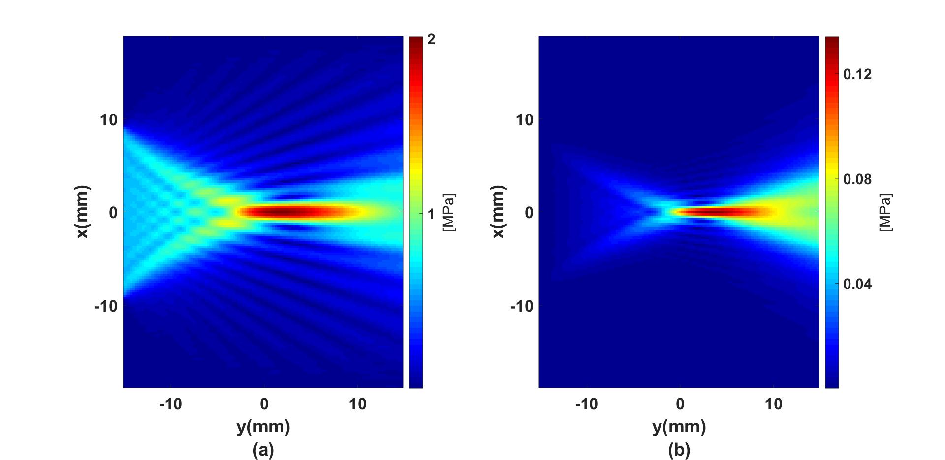
2D forward simulation

The fundamental pressure field is calculated with the 2D forward simulation function Forward2D_fund. The pressure field at the second-harmonic frequency under the quasi-linear approximation (weakly nonlinear wave propagation) is calculated with the function Forward2D_sec.


% forward propagation of the fundamental pressure   
P_fundamental = Forward2D_fund(mgrid, medium, excit_p, omega_c, 0, 'NRL');

% forward propagation of the second-harmonic pressure   
P_second = Forward2D_sec(mgrid, medium, P_fundamental, omega_c, 'NRL');

fundamental and the second-harmonic pressure field generated with the phased array

Other examples