Simulation of a 2D homogeneous medium using the transient mixed domain method

This example demonstrates how to simulate wave propagation in a 2D homogeneous medium using the transient mixed domain method. A focused beam is simulated.

Generating the grid structure to define the computational domain

We first need to define the temporal and spatial domains in 2D forward simulations with the function set_grid. For 2D problems, six inputs are required to call this function. Coordinates defined within the mgrid structure are all in the Cartesian coordinates. In mSOUND simulations, the spatial resolution (dx for 2D; dx and dy for 3D) and the marching step size (dy for 2D; dz for 3D) should in principle be a small fraction of the wavelength (e.g., 1/4 of the smallest wavelength) for stability and accuracy, and it is common to have a marching step size different from the spatial resolution. One exception is that for homogeneous and linear media, the step size can be arbitrarily large. The temporal resolution should at least satisfy the Nyquist criteria. In practice, the best course of action is to have a convergence study conducted to determine the proper step size, spatial and temporal resolutions.

        
dx = 3.75e-04;    % step size in the x direction [m] 
dy = 3.75e-04;    % step size in the y direction [m] 
dt = 6.25e-08;    % time step size [s] 

x_length = 0.0454;   % computational domain size in the x direction [m] 
y_length = 0.0240;   % computational domain size in the y direction [m] 
t_length = 6e-05;    % temporal domain size [s] 
mgrid = set_grid(dt, t_length, dx, x_length, dy, y_length);

Defining the phased array transducer

In this example, a phased array transducer is used to generate the focused ultrasound beam.


fc = 1.0e6;            % fundamental frequency [Hz]   
TR_focus  = 0.0180;    % transducer focal length [m]         
TR_radius = 0.0090;    % transducer aperture radius [m]  

% calculate the phase delay  
delay = sqrt((mgrid.x).^2 + TR_focus^2)/medium.c0;  
delay = delay - min(delay);

Excitation signal

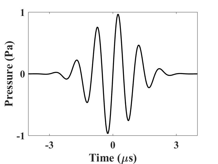
A four-cycle Gaussian-modulated pulse is used for the excitation signal. The pulse is illustrated in the figure below.


ts = [-4/fc:dt:4/fc].';   % define the pulse length [s]  
delay = repmat(delay, length(ts), 1);    
ts = repmat(ts, 1, mgrid.num_x);  

% define the excitation pulse   
p0 = 1; 
source_p = p0*sin(2*pi*fc*(ts+delay)).*exp(-(ts+delay).^2*fc^2/2); 
source_p(:, abs(mgrid.x)>TR_radius) = 0;

Defining the medium properties

Define the homogeneous medium. For 2D simulations, the medium properties should be given as matrices with a size (mgrid.num_x, mgrid.num_y+1). For homogeneous media, though, the medium properties can be described by a single scalar. medium.c0 is the reference speed of sound and generally, it is chosen as the minimum value of medium.c. When the power law exponent is 2.0(thermo-viscous losses), dispersion becomes absent.

  
medium.c    = 1500;    % speed of sound [m/s]      
medium.rho  = 1000;    % density [kg/m^3]             
medium.beta = 0;       % nonlinearity coefficient     
medium.ca   = 0;       % attenuation coefficient [dB/(MHz^y cm)]     
medium.cb   = 2.0;     % power law exponent    

% non-reflecting layer 
medium.NRL_gamma = 0.5;  
medium.NRL_alpha = 0.05;

2D forward simulation

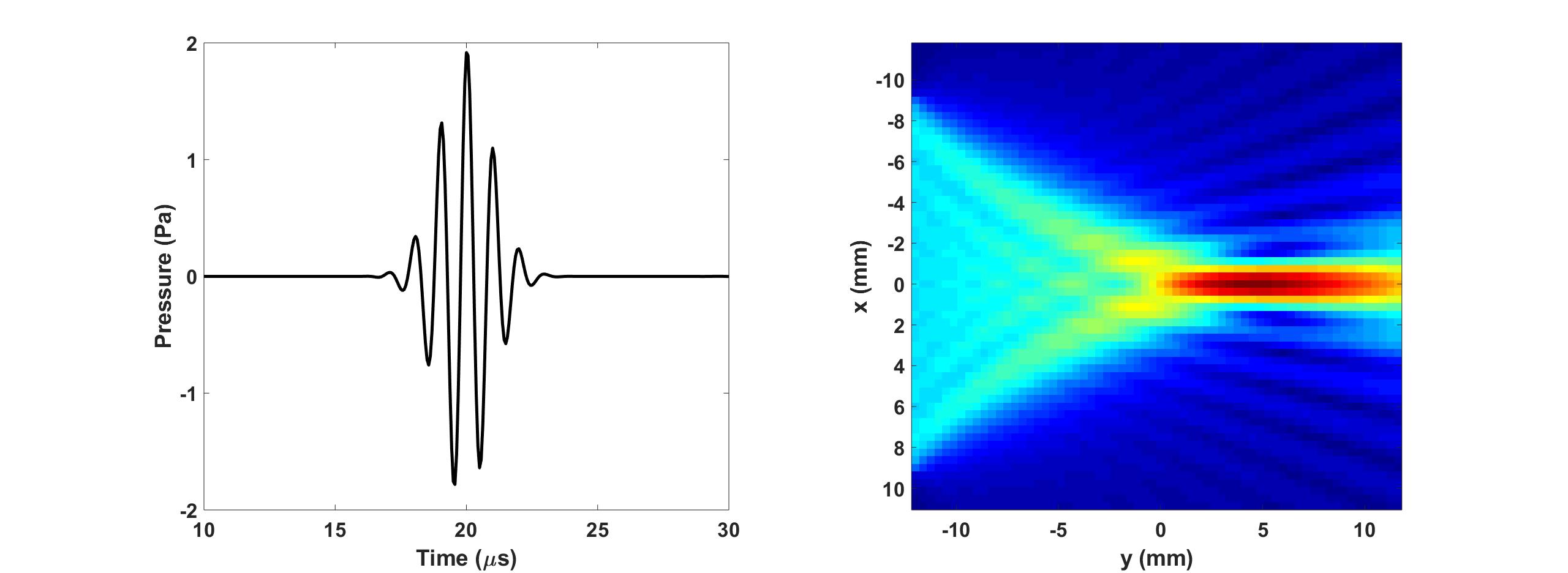
The pressure field is calculated with the 2D forward simulation function Forward2D. The waveform recorded at the transducer focal point and the center frequency pressure field distribution are shown below.


% define where the pressure will be recorded  
sensor_mask = zeros(mgrid.num_x, mgrid.num_y+1);
sensor_mask(30:90,2:end) = 1;  

% 2D forward simulation  
p = Forward2D(mgrid, medium, source_p, sensor_mask, 0, 'NRL');

(a) Time-domain singal recorded at the transducer focus (b) Fundamental pressure distribution through the sensor mask

Other examples