Reconstruction of the source pressure distribution with FSMDM in a 3D homogeneous medium

In this example, the pressure distribution on the source plane is reconstructed by using the backward projection with FSMDM. This is essentially the process of acoustical holography. In this manner, a field measured away from a transducer could be used to predict field behavior closer to the radiator or on the surface of the radiator. Alternatively, a desired field could be synthetically generated and then projected backward to provide information on the requirement of the radiational and dimensional requirements of the source. When using the FSMDM for backward projection, this process requires the frequency-domain information of a sound field over a given plane as well the acoustic properties of the propagation medium. Note that acoustical holography can also be implemented with the TMDM (by using Backward3D), where the process requires the time history of a sound field over a given spatial plane as well as the acoustic properties of the medium.

Generating the grid structure to define the computational domain

We first need to define the temporal and spatial computational domains in 3D forward simulations. In FSMDM, any arbitrary values can be set for the time step and temporal domain size, since they are not being used. Here, we set them to 0.

      
dx = 1.8750e-04;   % step size in the x direction [m] 
dy = 1.8750e-04;   % step size in the y direction [m] 
dz = 0.0210;       % step size in the z direction [m] 

x_length = 0.0450;   % computational domain size in the x direction [m] 
y_length = 0.0450;   % computational domain size in the y direction [m] 
z_length = 0.0210;   % computational domain size in the z direction [m] 
    
mgrid = set_grid(0, 0, dx, x_length, dy, y_length, dz, z_length);

Forward propagation

This example is based on the example Simulation of a 3D homogeneous medium using the frequency-specific mixed domain method The source pressure distribution is defined as shown below (four piston transducers).


% define the source   
X = (ones(mgrid.num_y,1)*mgrid.x).';
Y = ones(mgrid.num_x,1)*mgrid.y;
RHO = sqrt(X.^2+Y.^2);

source_map1 = sqrt((X-lambda*3).^2 + (Y+lambda*3).^2);   
source_map2 = sqrt((X+lambda*3).^2 + (Y+lambda*3).^2); 
source_map3 = sqrt((X-lambda*3).^2 + (Y-lambda*3).^2); 
source_map4 = sqrt((X+lambda*3).^2 + (Y-lambda*3).^2); 

% radius of each piston transducer  
TR_radius = 0.0037; 

source_map1(source_map1<=TR_radius) = 1;
source_map2(source_map2<=TR_radius) = 1;
source_map3(source_map3<=TR_radius) = 1;
source_map4(source_map4<=TR_radius) = 1;
source_map = source_map1  + source_map2 + source_map3 + source_map4;
source_map(source_map<1)=0;
p0 = 1; % pressure amplitude[Pa] 
source_p = p0*source_map;

3D forward simulation

The pressure field on a plane 21 mm away from the source plane is first calculated with the function Forward3D_fund.

 
omega_c = 2*pi*fc;
reflection_order = 0;
% forward propagation    
p = Forward3D_fund(mgrid, medium, source_p, ...
    omega_c, reflection_order, 'NRL');

Reconstruction

The source plane pressure distribution is obtained with the function Backward3D_fund.

 
reflection_order = 0;
source_p = p(:,:,end);
% backward propagation    
p = Backward3D_fund(mgrid, medium, source_p, ...
                omega_c, reflection_order, 'NRL');

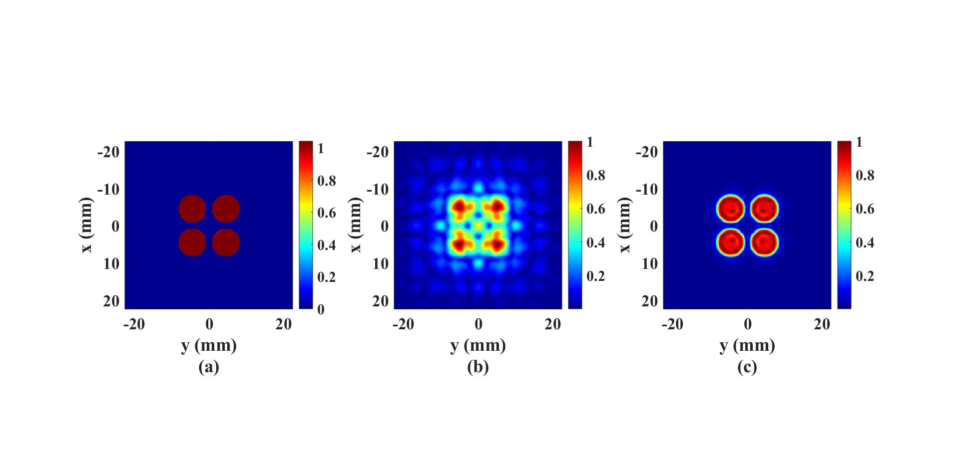
The figure below shows (a) ground-truth pressure distribution, (b) pressure distribution on the xy plane 21 mm away from the source plane and (c) the reconstructed source plane pressure distribution. It should be noted that mSOUND does not automatically allows near-field acoustic holography, as the evanescent waves are filtered out during the backward propagation. To disable this filter, the user can go to Backward3D_fund.m and comment out all the lines with the format F(real(Ktemp1)<=0) = 0. In this way, subwavelength information can be restored from the backward projection. (a) ground-truth source distribution,
(b) pressure distribution at the xy plane 21 mm away from the source plane
and (c) the reconstructed source pressure distribution

(a) ground-truth source distribution,
(b) pressure distribution at the xy plane 21 mm away from the source plane
and (c) the reconstructed source pressure distribution

Other examples