Simulation of a 2D heterogeneous medium using the transient mixed domain method

This example demonstrates how to use the transient mixed domain method for simulating wave propagation in 2D heterogeneous media.

Defining the medium properties

The setup of the computational domain and transducer in this example is similar to that in Simulation of a 2D homogeneous medium using the transient mixed domain method. All relevant acoustical properties including the speed of sound, density, nonlinearity coefficient, attenuation coefficient and power law exponent can vary in space in order to model truly heterogeneous media. medium.c0 is defined as the minimum value in the medium.c. The 2D tissue model used in this example is shown in the figure below. The red line on the left boundary indicates the array position. The red dot is the geometrical focus.

 
p0 = 1.0e6;    % source pressure magnitude [Pa]  
fc = 1.0e6;    % fundamental frequency [Hz]  
TR_focus  = 0.0210;    % transducer focal length [m]         
TR_radius = 0.0112;    % Transducer radius [m] 

load tissue_model.mat   % load the tissue model data   
medium.c    = c;        % speed of sound [m/s]      
medium.rho  = rho;      % density [kg/m^3]             
medium.beta = beta;     % nonlinearity coefficient     
medium.ca   = ca;       % attenuation coefficient [dB/(MHz^y cm)]     
medium.cb   = cb;       % power law exponent 
medium.c0 = min(min(c));  % reference speed of sound [m/s] 

medium.NRL_gamma = 0.5;
medium.NRL_alpha = 0.05;

2D forward simulation

The acoustic pressure field is calculated with the 2D forward simulation function Forward2D.


% define where the pressure will be recorded  
sensor_mask = zeros(mgrid.num_x, mgrid.num_y+1);
sensor_mask(100:300, 2:end) = 1;

% the maximum order of reflection included in the simulation  
reflection_order = 2; 

% 2D forward simulation  
p_total = Forward2D(mgrid, medium, source_p, sensor_mask, reflection_order, 'NRL');

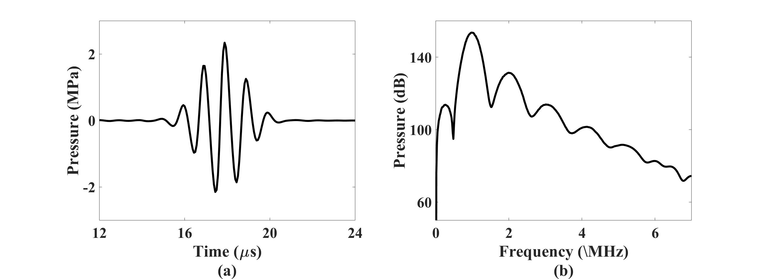
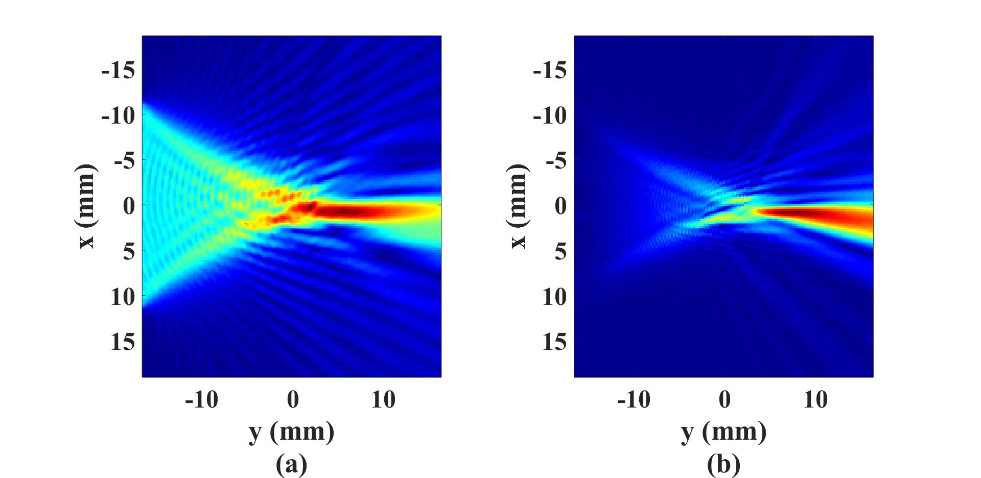
The acoustic signal recorded at the transducer focus as well as its Fourier components are shown in the top two figures shown below. Acoustic pressure fields at the fundamental and the second-harmonic frequencies are shown in the bottom two figures. time and frequency domain signal at the transducer focus

Other examples