Comparing rigid boundary condition and pressure release boundary condition for modeling ultrasound transducers

This example illustrates the difference between the rigid boundary condition (baffled source) and pressure release boundary condition for modeling ultrasound transducers. Currently, mSOUND uses the pressure release boundary condition, in which the planar transducer surface is assigned with a certain pressure distribution and the pressure is zero everywhere else on the input plane. When modeling a baffled source, where the rigid boundary condition is assumed, the transducer is assigned with a certain particle velocity distribution and the particle velocity in the normal direction is zero everywhere else. These two boundary conditions normally would produce different results mainly in the near-field, but the difference becomes less significant in the far-field. In this example, we use mSOUND to model a planar transducer with the pressure release boundary condition. We also use mSOUND to model the same transducer with the rigid boundary condition. In this case, the input plane pressure is obtained from FOCUS. The flat transducer has a diameter of 20 mm.

Generating the grid structure to define the computational domain

We first need to define the temporal and spatial computational domains in 3D forward simulations. In FSMDM, any arbitrary values can be set for the time step and temporal domain size, since they are not being used. Here, we set them to 0. We also define the background acoustic medium in this section.

      

medium.c0 = 1500;       % speed of Sound [m/s] 
medium.rho0 = 1000;     % density of medium [kg/m^3] 
medium.ca0 = 0;         % attenuation coefficient [dB/(MHz^y cm)]; 1 dB/cm at 500 kHz  
medium.cb0 = 2.0;       % power law exponent   

dx = lambda/6;   % step size in the x direction [m] 
dy = lambda/6;   % step size in the y direction [m] 
dz = lambda/6;   % step size in the z direction [m] 

x_length = 70e-3*4+dx;     % computational domain size in the x direction [m] 
y_length = 70e-3*4+dx;     % computational domain size in the y direction [m] 
z_length = 120e-3-19*dz;   % computational domain size in the z direction [m] 
    
mgrid = set_grid(0, 0, dx, x_length, dy, y_length, dz, z_length);

Excitation signal

We assume pressure release boundary in the first simulation. In the 2nd simulation, the input plane pressure is generated by FOCUS, which uses the rigid boundary condition. The corresponding FOCUS code (input_plane_FOCUS_unfocused_transducer_code.m) can be found in the example folder.

  
 % set up pressure release boundary condition  
source_p = p0*ones(mgrid.num_x,mgrid.num_y);   
 % set the pressure to be zero outside the source surface  
source_p(RHO>TR_radius) = 0; 

 % load FOCUS input plane pressure  
load FOCUS_input_plane_unfocused_lossless_0.5mm.mat
source_p1 = p_amp.*exp(1i*p_phase);

Defining the medium properties

Define the homogeneous medium. It is the same as the background medium.

 
medium.c    = medium.c0;     % speed of sound [m/s]   
medium.rho  = medium.rho0;   % density [kg/m^3]                
medium.ca   = medium.ca0;    % attenuation coefficient [dB/(MHz^y cm)]     
medium.cb   = medium.cb0;    % power law exponent  

% setting the non-reflecting boundary layer    
medium.NRL_gamma = 0.1;  
medium.NRL_alpha = 0.02;

3D forward simulation

The pressure field is calculated with the 3D forward simulation function Forward3D_fund.

 
fc = 0.5e6;        % ultrasound frequency/ Hz   
omega_c = 2*pi*fc; % angular frequency   
% forward propagation of the wave at the fundamental frequency 
%for the two boundary conditions    
[P_fundamental] = Forward3D_fund(mgrid, medium, source_p, omegac, 0 ,[],'NRL');
[P_fundamental1] = Forward3D_fund(mgrid, medium, source_p1, omegac, 0 ,[],'NRL');

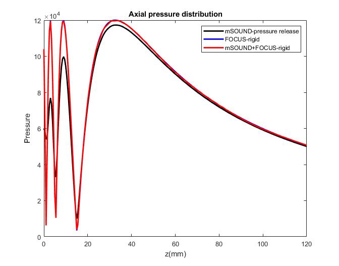
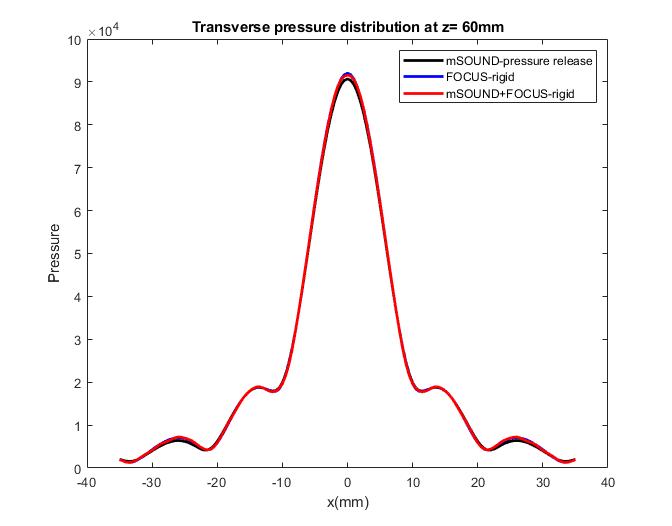
The two figures below show the pressure field distribution along the axial direction and transverse direction (at 60 mm depth). The results obtained from FOCUS alone (blue line) are also shown for comparison. As expected, the difference between the two different boundary conditions mainly exist in the near field. This difference must be considered when comparing mSOUND with other solvers. Axial pressure field of the flat transducer

Axial pressure field of the flat transducer

Transverse pressure field of the flat transducer

Other examples