Integrating mSOUND with k-Wave for transducers of curved shape

This example shows how to integrate mSOUND with k-Wave for simulations involving curved transducers. Currently, only planar phased-arrays can be directly set up in mSOUND for modeling focused beams. To more accurately model a physically curved transducer, the user needs to first use k-Wave (or other software such as FOCUS, Field II, etc.) to propagate the wave field from the curved transducer for a small distance and record the pressure field on a plane. The recorded pressure field can be then used as the input to mSOUND to further propagate the sound. In this example, a 2D curved transducer is first modeled with k-Wave and then with mSOUND.

Defining the computational domain in k-Wave

Define the computational domain in the k-Wave calculation.

         
dx = 1.8750e-04;   % step size in the x direction [m] 
dy = 1.8750e-04;   % step size in the y direction [m] 
dt = 3.1250e-08;   % time step size [s] 

Nx = 240;   % computational domain size in the x direction [grid points] 
Ny = 50;    % computational domain size in the y direction [grid points] 
kgrid = kWaveGrid(Nx, dx, Ny, dy);     

fc = 1.0e6;  % fundamental frequency [Hz]
kgrid.t_array = 0:dt:40/fc;  % time array [s]

Defining a curved transducer in k-Wave

In this example, a curved transducer is defined in k-Wave using the function makeCircle.

  
TR_radius = 0.0120;   % transducer aperture radius [m]  
TR_focus  = 0.0150;   % transducer focal length [m]       
focus  = round(TR_focus/dx);    % transducer focal length [grid points]   
cx = round(Nx/2);  % x coordinate of the transducer center[grid points]    
cy = 10 + focus;   % y coordinate of the transducer center[grid points]    

arc_angle1 = asin(TR_radius/TR_focus);  % [radians]      
arc_angle2 = pi*2;                      % [radians]     
arc_angle3 = pi*2 - arc_angle1;         % [radians]     
circle1    = makeCircle(Nx, Ny, cx, cy, focus, arc_angle1, false);
circle2    = makeCircle(Nx, Ny, cx, cy, focus, arc_angle2, false);
circle3    = makeCircle(Nx, Ny, cx, cy, focus, arc_angle3, false);
circle     = circle2 - circle3 + circle1;

source.p_mask = zeros(Nx, Ny);
source.p_mask = circle;  % define source mask    
sensor.mask   = zeros(Nx, Ny); 
sensor.mask(:, Ny/2+offcenter) = 1;  % define sensor mask

Excitation signal

A four-cycle Gaussian-modulated pulse is used as the excitation signal.

   
source_mag = 1;  % [Pa]    
ts = [-num_cycles/fc:dt:num_cycles/fc];   % excitation pulse length    
excit_p = sin(2*pi*fc*(ts)).*exp(-(ts).^2*fc^2/2);   % excitation pulse     
source.p = excit_p*source_mag;

input_args  = {'DisplayMask', source.p_mask, 'DataCast', 'single'};
% run the simulation   
sensor_data = kspaceFirstOrder2D(kgrid, medium, source, sensor, input_args{:});
% reshape the output data for further simulation   
sensor_data = reshape(sensor_data, Nx, length(kgrid.t_array));

Implementing signals to the TMDM

Pressure recorded at the sensor positions from the k-Wave simulation will be used as the source pressure in mSOUND. It is noted that sensor data from k-Wave is indexed as [time, sensor_positions], while in mSOUND it is [sensor_positions, time]. If the time step or transverse spatial domain size in k-Wave is different from that in mSOUND, sensor_data from the k-Wave needs to be resized.

 
% defining the computational domain in mSOUND  
x_length = kgrid.dx*kgrid.Nx;
y_length = TR_focus - kgrid.dy*(Ny-20);
t_length = max(kgrid.t_array); 
dt = 6.2500e-08;  % time step in mSOUND [s]  
mgrid = set_grid(dt, t_length, dx, x_length, dy, y_length);  

% resize the sensor data as a larger time step is applied in mSOUND  
source_p = sensor_data(:, 1:2:end).'; 

% Define the medium properties in the TMDM   
medium.c    = 1500;   % speed of sound [m/s]   
medium.rho  = 1000;   % density [kg/m^3]   
medium.beta = 0.0;    % nonlinear coefficient   
medium.ca   = 0;      % attenuation coefficient [dB/(MHz^y cm)]      
medium.cb   = 2.0;    % power law exponent   
medium.c0   = 1500;   % reference speed of sound [m/s]

Forward simulation with TMDM

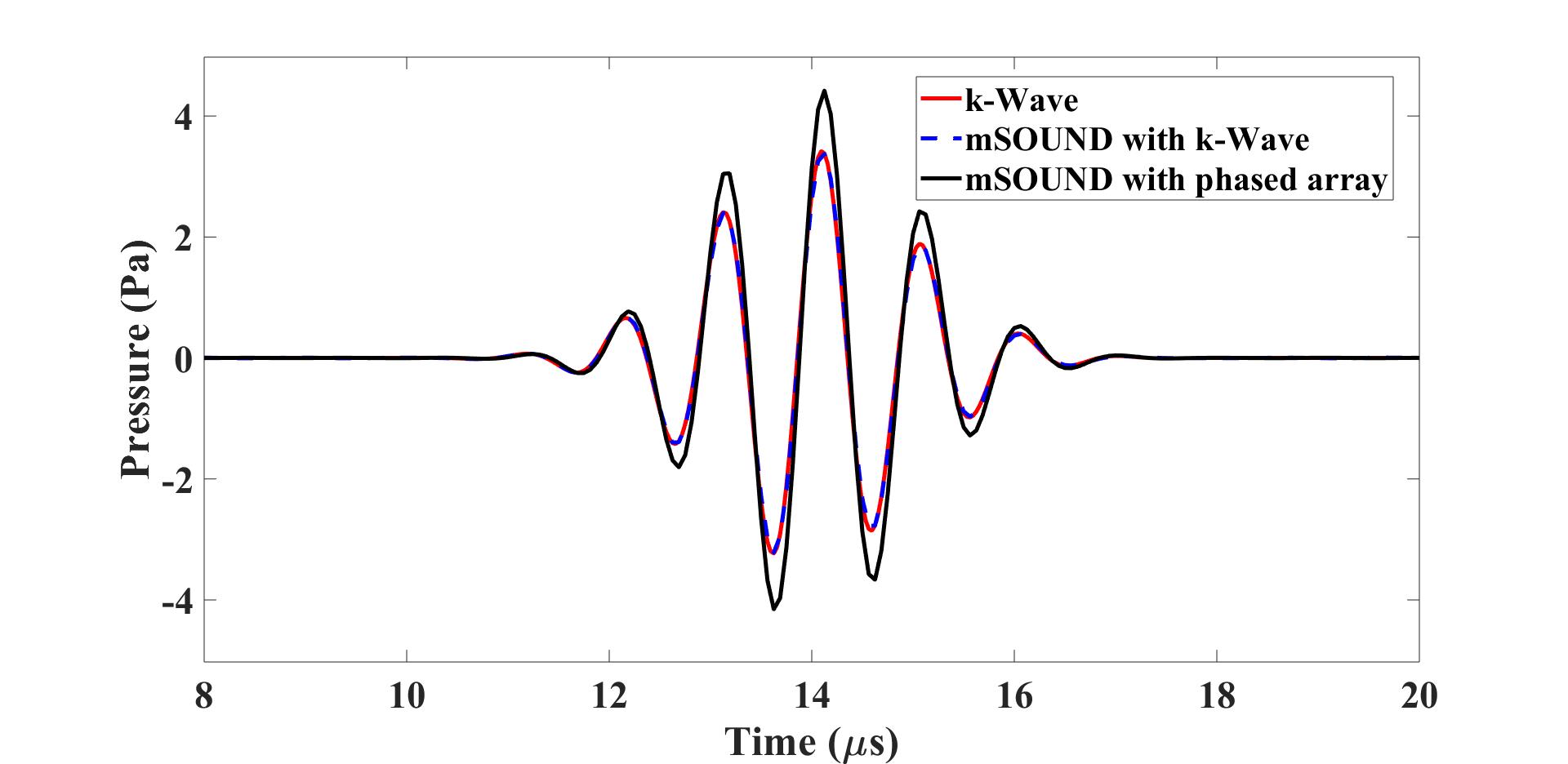
The figure below shows the waveform at the geometrical focus of the transducer. The result generated with mSOUND is compared with the result directly simulated with k-Wave and excellent agreement can be seen. The result generated with mSOUND using a phased array is also compared in this figure.

 
 % define sensor mask in mSOUND   
sensor_mask = zeros(mgrid.num_x, mgrid.num_y+1);
sensor_mask(:, end) = 1;

% 2D forward simulation with mSOUND   
reflection_order = 0;
p_time = Forward2D(mgrid, medium, source_p, sensor_mask, reflection_order);

Time-domain singal recorded at the transducer focus

Other examples