Shock wave simulations with TMDM

Due to the lack of a shock-capturing algorithm, mSOUND is currently not ideal for modeling shock waves. Shock waves, however, can still be modeled with either very fine step size, spatial and temporal resolutions, or by using artificial attenuations to dampen the excessive high frequency components. This example demonstrates how to model a shock wave using TMDM and it is extended from Simulation of a 2D homogeneous medium using the transient mixed domain method.

Generating the grid structure to define the computational domain

We first need to define the temporal and spatial domains in 2D forward simulations with the function set_grid. A relatively small temporal domain size is used in this example to reduce the computation (please refer to the example Selecting the proper temporal domain size for the TMDM). Three cases are studied in this example. In the first case, we have medium.ca = 0.02, dy = 1.5000e-06 and dt = 1.0000e-09 (so that 500 harmonics are considered). In the second case, we increase dy and dt, so that dy = 7.5000e-06 and dt = 5.0000e-09 (100 harmonics are considered). In the third case, we artificially increase the attenuation so that dy = 7.5000e-06, dt = 5.0000e-09 and medium.ca = 0.1. The simulation setup for the first case is shown below.

        
dx = 1.8750e-04;    % step size in the x direction [m] 
dy = 1.5000e-06;    % step size in the y direction [m] 
dt = 1.0000e-09;    % time step size [s] 

x_length = 0.0454;      % computational domain size in the x direction [m] 
y_length = 0.0240;      % computational domain size in the y direction [m] 
t_length = 1.6000e-05;  % temporal domain size [s] 
mgrid = set_grid(dt, t_length, dx, x_length, dy, y_length);

Excitation signal

A sine wave is used as the excitation signal.

 
ts = [0:dt:16/fc].';   % define the excitation signal length [s]  
delay = repmat(delay, length(ts), 1);    
ts = repmat(ts, 1, mgrid.num_x);  

p0 = 6.5e6;   % pressure magnitude [Pa]  
source_p = p0*sin(2*pi*fc*(ts+delay)); 
source_p(:, abs(mgrid.x)>TR_radius) = 0;

Defining the medium properties

  
medium.c    = 1500;    % speed of sound [m/s]      
medium.rho  = 1000;    % density [kg/m^3]             
medium.beta = 3.6;     % nonlinearity coefficient     
medium.ca   = 0.02;   % attenuation coefficient [dB/(MHz^y cm)]     
medium.cb   = 2.0;     % power law exponent

2D forward simulation

The pressure field is calculated with the function Forward2D.


% define where the pressure will be recorded  
sensor_mask = zeros(mgrid.num_x, mgrid.num_y+1);
sensor_mask(round(mgrid.num_x/2), focus+1) = 1;  

% 2D forward simulation  
p = Forward2D(mgrid, medium, source_p, sensor_mask, 0);

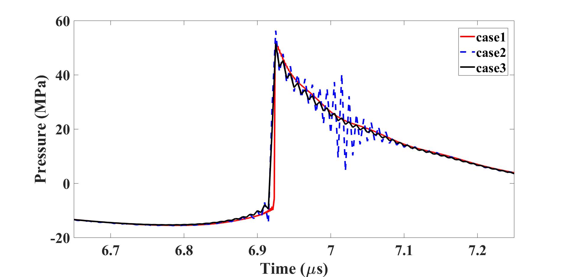
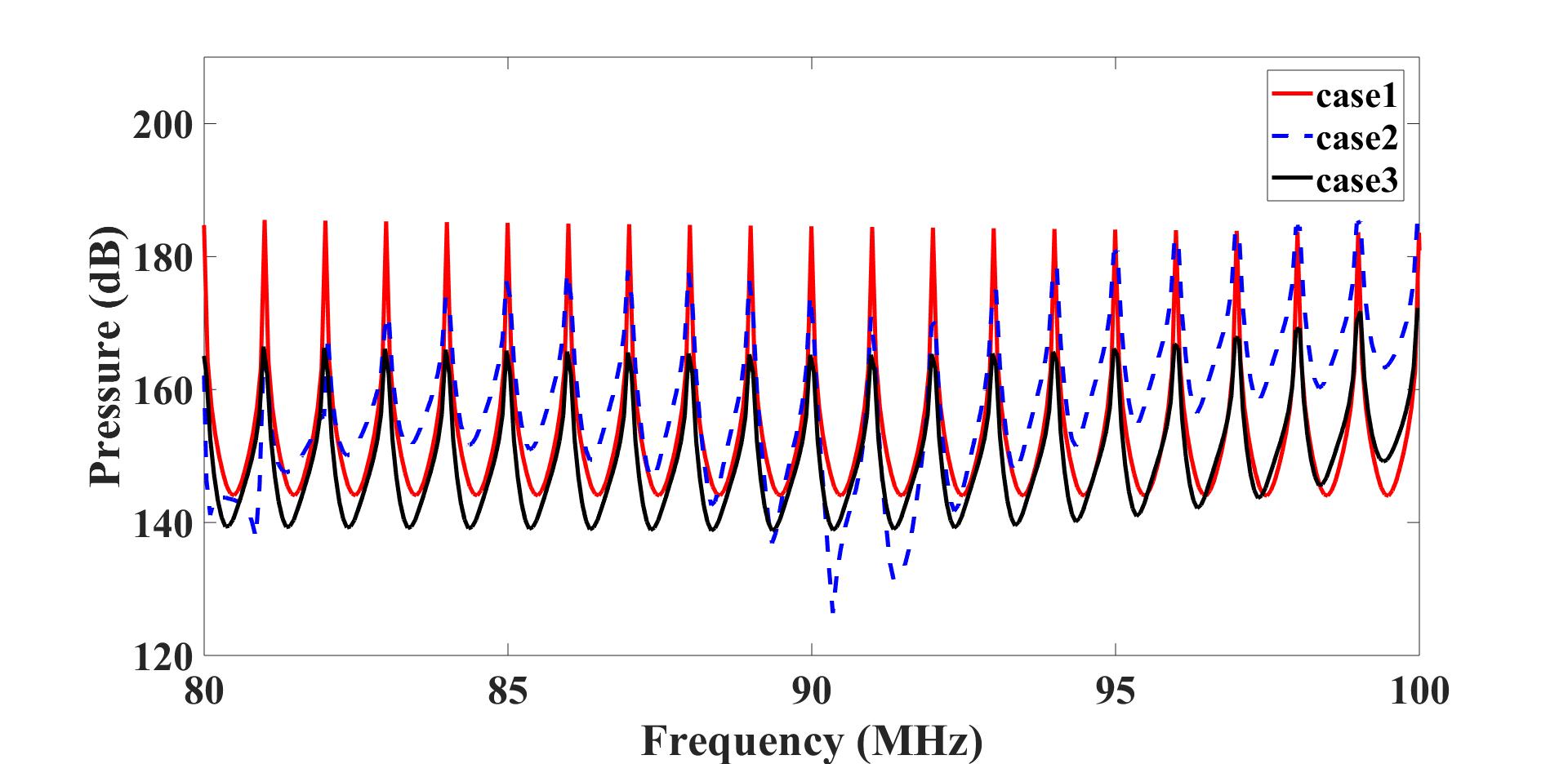
The figures below compare the simulation results from the three different cases. The first figure compares the waveforms recorded at the transducer focus and the second figure compares the frequency-domain spectra (only the high frequency components are shown). Case 1 yields satisfactory results due to the fine step size, spatial resolution, and temporal resolution. It is therefore considered as the benchmark here. With the artificial attenuation, the shock-front can be captured reasonably well with a fairly large step size and coarse temporal resolution (case 3), while the one without the artificial attenuation produces large a Gibbs noise (case 2). In this example, the simulation time for case 3 is around 24 times faster than that of case 1. time-domain results

Other examples