One step reconstruction of the source pressure distribution with FSMDM in a 3D homogeneous medium

This example shows that when reconstrcting the pressure distribution in homogeneous medium, the step size can be chosen as large as the propagation distance. Results in this example are compared with the results in Reconstruction of the source pressure distribution with FSMDM in a 3D homogeneous medium, in which a smaller step size is used. Simulation step up are very similar in these two examples.

Generating the grid structure to define the computational domain

We first need to define the temporal and spatial computational domains in 3D forward simulations. In FSMDM, any arbitrary values can be set for the time step and temporal domain size, since they are not being used. Here, we set them to 0.

      
dx = 1.8750e-04;   % step size in the x direction [m] 
dy = 1.8750e-04;   % step size in the y direction [m] 
dz = 0.0210;       % step size in the z direction [m] 

x_length = 0.0900;   % computational domain size in the x direction [m] 
y_length = 0.0900;   % computational domain size in the y direction [m] 
z_length = 0.0210;   % computational domain size in the z direction [m] 
    
mgrid = set_grid(0, 0, dx, x_length, dy, y_length, dz, z_length);

3D forward simulation

The pressure field on a plane 21 mm away from the source plane is first calculated with the function Forward3D_fund. In this example, the spatial aliasing errors are reduced by increasing the transverse domain size, while in the example Reconstruction of the source pressure distribution with FSMDM in a 3D homogeneous medium, absorbing layers are used. The reason we choose to increase the domain size here is because, in the one-step reconstruction/projection case, the absorption layer is not effective anymore. The absorption layer can only be modeled accurately by marching the wave field step-by-step in the z-direction (3D) or y-direction (2D).

 
omega_c = 2*pi*fc;
reflection_order = 0;
% forward propagation    
p = Forward3D_fund(mgrid, medium, source_p, omega_c, reflection_order);

Reconstruction

The source plane pressure distribution is obtained with the function Backward3D_fund.

 
source_p = p(:,:,end);
% backward propagation    
p = Backward3D_fund(mgrid, medium, source_p, omega_c, reflection_order);

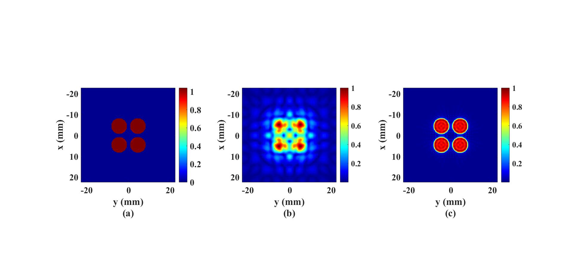
The figure below was generated with the one-step recostruction method and it shows (a) ground-truth pressure distribution, (b) pressure distribution on the xy plane 21 mm away from the source plane and (c) the reconstructed source plane pressure distribution. (a) ground-truth source distribution,
(b) pressure distribution at the xy plane 21 mm away from the source plane
and (c) the reconstructed source pressure distribution

(a) ground-truth source distribution,
(b) pressure distribution at the xy plane 21 mm away from the source plane
and (c) the reconstructed source pressure distribution

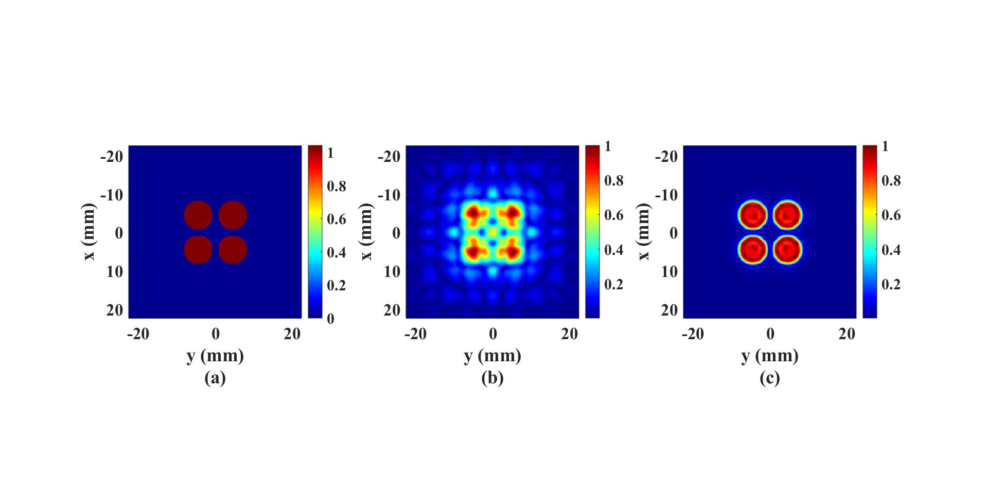
The figure below was generated with the simulation setup shown in the example Reconstruction of the source pressure distribution with FSMDM in a 3D homogeneous medium and it shows (a) ground-truth pressure distribution, (b) pressure distribution on the xy plane 21 mm away from the source plane and (c) the reconstructed source plane pressure distribution. (a) ground-truth source distribution,
(b) pressure distribution at the xy plane 21 mm away from the source plane
and (c) the reconstructed source pressure distribution

Other examples